A3C、PPO、GAE笔记

一、重要性采样

TRPO和PPO主要思想的数学基础是重要性采样

重要性采样：$x_i $是从$p(x)$分布中采样得到的，但是$p(x)$的值往往无法直接获得，需要通过其他分布$q(x)$进行间接采样获得。

$\begin{aligned} \mathbb{E}_{x\sim p}[f(x)] &=\int f(x)p(x) dx \\ &=\int f(x) \frac{p(x)}{q(x)}q(x)dx \\ &=\mathbb{E}_{x\sim q}[f(x)\frac{p(x)}{q(x)}] \end{aligned}$

条件：
- $p$分布与$q$分布需要相近，才能得到较好的效果。
用在强化学习里面:
- 由于策略梯度原始公式中的新策略分布难以得到，因而使用旧策略进行间接采样，以使得未知项变成可估计的已知项进行计算。

二、梯度与参数更新

1. 回报的期望：最大化全部采样轨迹上的策略回报值，$R(\tau)$ 表示某一个轨迹$\tau$的回报值

$argmax_\theta \space \mathbb{E}[{R_\theta}]=\sum_\tau R(\tau)p_\theta(\tau)$

2. 回报的期望的梯度：(第三个等号用到的公式：$\nabla f(x) = f(x) \nabla \log f(x)$)

$\begin{aligned} \nabla \mathbb{E}[{R_\theta}]&=\sum_\tau R(\tau) \nabla p_{\theta}(\tau) \\ &= \sum_\tau R(\tau)p_\theta(\tau)\frac{\nabla p_\theta(\tau)}{p_\theta(\tau)} \\ &= \sum_\tau R(\tau)p_\theta(\tau){\nabla \log p_\theta(\tau)}\\ &= \mathbb{E}_{\tau \sim p_\theta{(\tau)}}[R(\tau){\nabla \log p_\theta(\tau)}] \\ &≈ \frac{1}{N} \sum_{n=1}^{N}R(\tau^n)\nabla \log p_{\theta}(\tau^n) \\ &=\frac{1}{N}\sum_{n=1}^{N} \sum_{t=1}^{T_n} R(\tau^n)\nabla \log p_\theta(a_t^n|s_t^n) \end{aligned}$

式中

$N$表示采样了$N$条trajectory, $T_n$表示每条trajectory的step数量。
关于$p_{\theta}(\tau)$
$\begin{aligned} p_{\theta}(\tau) &= p(s_1)p_\theta(a_1|s_1)p(s_2|s_1,a_1)p_\theta(a_2|s_2)p(s_3|s_2,a_2) \space\space...\space\space \\ &=p(s_1) \prod_{t=1}^T p_{\theta}(a_t|s_t)p(s_{t+1}|s_t, a_t) \end{aligned}$
由两部分组成一部分是来自环境的 $p_\theta(s_{t+1}|s_t, a)$，一部分是来自agent的 $p_\theta {(a_t|s_t)}$, 其中来自环境的部分不带入计算，策略更新只考虑agent这部分。所以最后一步并没有$t+1$这部分。

3. 参数更新：

$\theta = \theta+\eta \nabla \bar{R_\theta}$

三、实际算法中对策略梯度的处理方法

策略梯度方法：

加入baseline
$\nabla \bar{R_\theta}=\frac{1}{N} \sum_{n=1}^{N}(R(\tau^n)-b)\nabla \log p_{\theta}(\tau^n) \\ b≈\mathbb{E}[R(\tau)]$

$b$ 的加入保证reward不是恒大于0的，若reward一直大于0，则会导致未被采样的action无法得到提升，但其实该action并不是不好而是未被采样。

状态值函数估计轨迹回报：

$R(\tau^n)-b$ 部分使用状态值函数来替代
$q(s,a)$
优势函数估计轨迹回报：

$R(\tau^n)-b$ 部分用以下Advantage function来替代

$A(s_t,a_t)= q(s,a)-V(s)$

TD-Error估计轨迹回报：(A3C)使用值网络估计值，引入bias减小variance

$R(\tau^n)-b$ 部分用以下TD-Error 代替
$r(s_t. a_t)+v(s_{t+1})-v(s)$

四、GAE(Generalized Advantage Estimation)

GAE的作用
- GAE的意思是泛化优势估计，因而他是用来优化Advantage Function优势函数的。
- GAE的存在是用来权衡variance和bias问题的：
  - On-policy直接交互并用每一时刻的回报作为长期回报的估计$\sum_{t’=t}^{T} \gamma^{t’-t}r_{t’}$ 会产生较大的方差，Variance较大。
  - 而通过基于优势函数的AC方法来进行回报值估计，则会产生方差较小，而Bias较大的问题。
GAE 推导

满足$\gamma$-just条件。(未完待续)
GAE形式

GAE的形式为多个价值估计的加权平均数。
$TD Error=\delta_t=r_t+\gamma v(s_{t+1})-v(s_t)$
运用GAE公式进行优势函数的估计：

$\sum_{l=0}^\infin(\gamma\lambda)^l \delta_{t+l}^V$

为了快速估计序列中所有时刻的估计值，采用倒序计算，从t+1时刻估计t时刻：

$\hat{A_t}^{GAE(\gamma,\lambda)}=\sum_{l=0}^{\infin}(\gamma\lambda)^l \delta_{t+l}^V=\delta_t^V+\gamma\lambda\hat{A}_{t+l}^{GAE(\gamma,\lambda)}$

五、PPO关于策略梯度的目标函数

以上所述的策略梯度算法属于on-policy的算法，而PPO属于off-policy的算法

on-policy: 使用当前策略$\pi_\theta$收集数据，当参数$\theta$更新后，必须重新采样。
$\nabla \bar{R_\theta}=\mathbb{E}_{\tau \sim p_\theta{\tau}}[R(\tau){\nabla \log p_\theta(\tau)}]$
off-policy: 可以从可重用的样本数据中获取样本来训练当前的策略$\pi _\theta$，下式用了重要性采样。
$\nabla \bar{R_\theta}=\mathbb{E}_{\tau \sim p_{\theta^\prime}{\tau}}[\frac{p_\theta(\tau)}{p_{\theta^\prime}(\tau)} R(\tau){\nabla \log p_\theta(\tau)}]$

1. PPO目标函数

对于PPO而言，轨迹回报通过采用Advantage function的方式进行估计，因而其梯度更新方式为：

$\begin{aligned} \nabla \bar{R_\theta} &=\mathbb{E}_{(s_t,a_t)\sim\pi_\theta}[A^\theta(s_t,a_t)\nabla \log p_\theta({a_t^n|s_t^n})] \\ &=\mathbb{E}_{(s_t,a_t)\sim\pi_\theta^\prime}[\frac{p_\theta(s_t,a_t)}{p_\theta^\prime(s_t,a_t)}A^{\theta^\prime}(s_t,a_t)\nabla \log p_\theta({a_t^n|s_t^n})] \\ &=\mathbb{E}_{(s_t,a_t)\sim\pi_\theta^\prime}[\frac{p_\theta(a_t|s_t)}{p_\theta^\prime(a_t|s_t)}\frac{p_\theta(s_t)}{p_\theta^\prime(s_t)}A^{\theta^\prime}(s_t,a_t)\nabla \log p_\theta({a_t^n|s_t^n})] \\ &≈\mathbb{E}_{(s_t,a_t) \sim \pi_\theta^\prime}[\frac{\nabla p_\theta(a_t|s_t)}{p_\theta^\prime(a_t|s_t)}A^{\theta^\prime}(s_t,a_t)] \end{aligned}$

其中，从第二个等式用的是重要性采样，第三到第四个约等式由于$\frac{p_\theta(s_t)}{p_\theta^\prime(s_t)}$这一项来源于重要性采样，前提假设两个分布差别不大，近似为1，且不易计算，故省略，后面的$\nabla \log p_\theta({a_t^n|s_t^n})$ ,根据公式$\nabla f(x) = f(x) \nabla \log f(x)$转换。

因而，定义目标函数为：

$J^{\theta^{\prime}} (\theta)=\mathbb{E}_{(s_t,a_t) \sim \pi_\theta^\prime}[\frac{p_\theta(a_t|s_t)}{p_\theta^\prime(a_t|s_t)}A^{\theta^\prime}(s_t,a_t)]$

2. PPO对于重要性采样约束的处理

为了保证$p_\theta(s_t,a_t) $ 与 $p_\theta^\prime(s_t,a_t)$ 分布的差别不会太大，采用以下约束：

TRPO：使用约束 $KL(\theta,\theta’)<\delta$，在分布上进行约束。
PPO1(Adaptive KL)：使用$J_{PPO}^{\theta’}(\theta)=J^{\theta’}(\theta)-\beta KL(\theta,\theta’)$，在目标函数上加一个正则项进行约束，注意，这里KL散度衡量的是action之间的距离，而不是参数$\theta$与$\theta’$之间的距离。
PPO2 (Clip，论文中推荐的)：使用$J_{PPO_2}^{\theta’}(\theta)=\sum_{(s_t,a_t)}\min\{([\frac{p_\theta(a_t|s_t)}{p_\theta^\prime(a_t|s_t)}A^{\theta^\prime}(s_t,a_t)], [clip(\frac{p_\theta(a_t|s_t)}{p_\theta^\prime(a_t|s_t)},1-\epsilon,1+\epsilon)A^{\theta^\prime}(s_t,a_t)])\}$, 来约束分布距离。

使用GAE对优势函数进行优化

def get_gaes(self, rewards, v_preds, v_preds_next):
    """
    GAE
    :param rewards: r(t)
    :param v_preds: v(st)
    :param v_preds_next: v(st+1)
    :return:
    """
    deltas = [r_t + self.gamma * v_next - v for r_t, v_next, v in zip(rewards, v_preds_next, v_preds)]

    #计算GAE(lambda = 1), 参见 ppo paper eq(11)
    gaes = copy.deepcopy(deltas)
    
    # 倒序计算GAE
    for t in reversed(range(len(gaes) - 1)):
        gaes[t] = gaes[t] + self.gamma * gaes[t + 1]
    return gaes

六、 PPO的目标函数

PPO的最终目标函数由三部分组成，可使用梯度下降求解，而不是像TRPO一样使用共轭梯度法：

策略梯度目标函数： $L_t^{CLIP}(\theta)$
值函数目标函数：$L_t^{VF}(\theta)=(V_\theta(s_t)-V_t^{target})^2=((r+\gamma v(s_{t+1}))-v(s_t))^2$
策略模型的熵: $S_{[\pi_\theta]}(s_t)=-\pi_\theta(a|s)\log\pi_\theta(a|s)$

完整的形式如下：

$L_t^{PPO_2}(\theta)=\hat{\mathbb{E}}_t[L_t^{CLIP}(\theta)-c_1L_t^{VF}(\theta)+c_2S_{[\pi_\theta]}(s_t)]$

这部分相应的代码如下：

with tf.variable_scope('assign_op'):
    self.assign_ops = []
    for v_old, v in zip(old_pi_trainable, pi_trainable):
        self.assign_ops.append(tf.assign(v_old, v))

# inputs for train_op
with tf.variable_scope('train_inp'):
    self.actions = tf.placeholder(dtype=tf.int32, shape=[None], name='actions')
    self.rewards = tf.placeholder(dtype=tf.float32, shape=[None], name='rewards')
    self.v_preds_next = tf.placeholder(dtype=tf.float32, shape=[None], name='v_preds_next')
    self.gaes = tf.placeholder(dtype=tf.float32, shape=[None], name='gaes')

act_probs = self.Policy.act_probs
act_probs_old = self.Old_Policy.act_probs

# agent通过新策略选择action的概率 probabilities of actions which agent took with policy
act_probs = act_probs * tf.one_hot(indices=self.actions, depth=act_probs.shape[1])
act_probs = tf.reduce_sum(act_probs, axis=1)

# agent通过旧策略选择action的概率 probabilities of actions which agent took with old policy
act_probs_old = act_probs_old * tf.one_hot(indices=self.actions, depth=act_probs_old.shape[1])
act_probs_old = tf.reduce_sum(act_probs_old, axis=1)

with tf.variable_scope('PPO_loss'):
    """
        策略目标函数
    """
    #
    # ratios = tf.divide(act_probs, act_probs_old)
    # r_t(θ) = π/πold 为了防止除数为0，这里截取一下值，然后使用e(log减法)来代替直接除法
    ratios = tf.exp(
        tf.log(tf.clip_by_value(act_probs, 1e-10, 1.0)) - tf.log(tf.clip_by_value(act_probs_old, 1e-10, 1.0)))
    # L_CLIP 裁剪优势函数值
    clipped_ratios = tf.clip_by_value(ratios, clip_value_min=1 - clip_value, clip_value_max=1 + clip_value)
    self.loss_clip = tf.minimum(tf.multiply(self.gaes, ratios), tf.multiply(self.gaes, clipped_ratios))
    self.loss_clip = tf.reduce_mean(self.loss_clip)

    """
        策略模型的熵
    """
    # 计算新策略πθ的熵 S = -p log(p) 这里裁剪防止p=0
    self.entropy = -tf.reduce_sum(
        self.Policy.act_probs * tf.log(tf.clip_by_value(self.Policy.act_probs, 1e-10, 1.0)), axis=1)
    self.entropy = tf.reduce_mean(self.entropy, axis=0)  # mean of entropy of pi(obs)

    """
        值目标函数
    """
    # L_vf = [(r+γV(π(st+1))) - (V(π(st)))]^2
    v_preds = self.Policy.v_preds
    self.loss_vf = tf.squared_difference(self.rewards + self.gamma * self.v_preds_next, v_preds)
    self.loss_vf = tf.reduce_mean(self.loss_vf)

    # construct computation graph for loss
    # L(θ) = E_hat[L_CLIP(θ) - c1 L_VF(θ) + c2 S[πθ](s)]
    # L = 策略目标函数 + 值目标函数 + 策略模型的熵
    self.loss = self.loss_clip - c_1 * self.loss_vf + c_2 * self.entropy
    # minimize -loss == maximize loss
    self.loss = -self.loss

optimizer = tf.train.RMSPropOptimizer(learning_rate=args.ppo_lr, epsilon=1e-5)
self.gradients = optimizer.compute_gradients(self.loss, var_list=pi_trainable)
self.train_op = optimizer.minimize(self.loss, var_list=pi_trainable)

七、Actor-Critic

A2C、A3C等方法采用的是TD方法来替代R-b部分

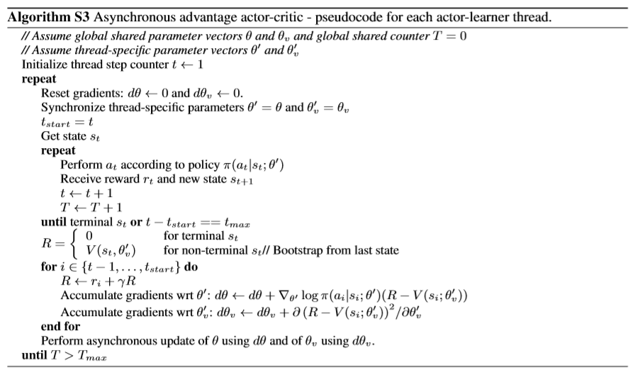
A3C
- 方法:
  - 启动N个线程，Agent在N线程中同时进行环境交互收集样本；
  - 收集完样本后，每一个线程将独立完成训练并得到参数更新量，异步更新到全局的模型参数中；
  - 下一次训练的时候，线程的模型参数将与全局参数完成同步，使用新的参数进行下一次训练。
- 目标函数:
  
  使用TD-$\lambda$减小TD带来的偏差，可以在训练早期更快的提升价值模型。为了增加模型的探索性，目标函数中引入了策略的熵。

$\nabla_\theta J(\theta)=\frac{1}{T}\sum_t^T\nabla_\theta \log \pi(a_t|s_t;\theta)(\sum_{i=0}^n\gamma^{i-1}r_{t+1}+v(s_{t+n})-v(s_t))+\beta\nabla_\theta H(s_t;\theta)$

A2C

与A3C不同的是参数更新全部在全局master完成，每个子线程只负责env.step()进行探索。

一、 重要性采样

二、 梯度与参数更新

三、 实际算法中对策略梯度的处理方法